Problem 10.13. Dynamic factor and dynamic load

Problem a)

Dynamic factor =

Dynamic load, p_dyn [N/m²]=

Problem b)

Dynamic factor =

Dynamic load, p_dyn [N/m²]=

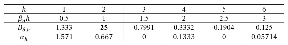
Step 1. Give the load in time by a Fourier series expansion

Check expansionHide expansion

The load in time is given by the following series:

Figure 358b, Eq.(10-105)

$$\begin{gathered} \tilde{p}\left(t\right)=p\left\{1+\sum _{h=1}^5{\alpha }_h\sin ({\varphi }_h+2\mathrm{\pi }h{f}_{p}t)\right\}, \\ {\alpha }_1=\frac{\mathrm{\pi }}{2}, {\alpha }_2=\frac{2}{3}, {\alpha }_3=0, {\alpha }_4=\frac{2}{15}, {\alpha }_5=0, {\alpha }_6=\frac{2}{35} \end{gathered}$$

Note that $p_1=p{\alpha }_1=186.5\frac{\mathrm{\pi }}{2}=293\frac{\mathrm{N}}{{\mathrm{m}}^2}$, which is the same as the load given in Problem 8.7. Also note that according to the solution of Problem 8.7 the contribution of the higher modes in space is marginal.

Step 2. Determine the first eigenfrequency of the slab

Check eigenfrequencyHide eigenfrequency

Eqs.(8-47), (8-1) or Problem 8.7

$f_n=f_1=\frac{{\omega }_1}{2\mathrm{\pi }}=\sqrt{\frac{{\mathrm{\pi }}^{2}EI}{4m{L}^4}}=4.415\frac{1}{\mathrm{s}}$

Problem a)

Step 3. Calculate the dynamic response for each term in time, disregarding the series expansion in space

Eqs.(10-115), (10-116)

${\beta }_n=\frac{f_p}{f_n}=\frac{2.5}{4.415}=0.5662$

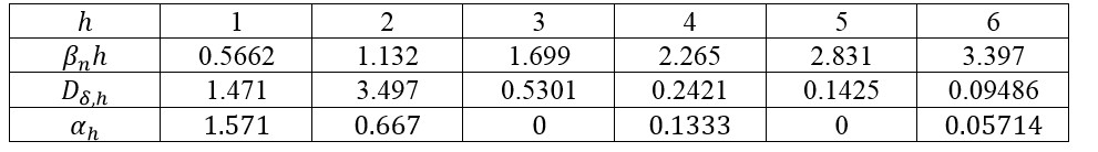
Step 4. Determine the dynamic factor

Eq.(10-115)

$1+\sum _{h=1}^5{\alpha }_h{D}_{\delta ,h}=1+2.311+2.331+0+0.03228+0+0.00542\mathbf{=}\mathbf{5}\mathbf{.}\mathbf{68}$

Step 5. Give the dynamic load

Eq.(10-115)

${\mathit{p}}_{\mathbf{dyn}}=p\left(1+\sum _{h=1}^H{\alpha }_h{D}_{\delta ,h}\right)\mathbf{=}\mathbf{1059}\frac{\mathbf{N}}{{\mathbf{m}}^{\mathbf{2}}}$

Problem b)

Step 3.

Calculate the dynamic response for each term in time, disregarding the series expansion in space

When the basic frequency may vary between 2 and 3 Hz, it is chosen in such a way that one of hf_p-s agrees with f_n, and hence due to resonance the response becomes high.

Figure 361

Now we set

$f_p=\frac{f_n}{2}=2.208\frac{1}{\mathrm{s}}$

The dynamic response is calculated for each term in time, disregarding the series expansion in space:

Eqs.(10-115), (10-116)

${\beta }_n=\frac{f_p}{f_n}=\frac{2.208}{4.415}=0.5$

Step 4. Determine the dynamic factor

Eq.(10-115)

$1+\sum _{h=1}^H{\alpha }_h{D}_{\delta ,h}=1+2.094+16.67+0+0.0444+0+00071\mathbf{=}\mathbf{19}\mathbf{.}\mathbf{81}$

Step 4. Give the dynamic load

Eq.(10-115)

${\mathit{p}}_{\mathbf{dyn}}=p\left(1+\sum _{h=1}^H{\alpha }_h{D}_{\delta ,h}\right)\mathbf{=}\mathbf{3695}\frac{\mathbf{N}}{{\mathbf{m}}^{\mathbf{2}}}$

The load in time is given by the following series:

Figure 358b, Eq.(10-105)

$$\begin{gathered} \tilde{p}\left(t\right)=p\left\{1+\sum _{h=1}^5{\alpha }_h\sin ({\varphi }_h+2\mathrm{\pi }h{f}_{p}t)\right\}, \\ {\alpha }_1=\frac{\mathrm{\pi }}{2}, {\alpha }_2=\frac{2}{3}, {\alpha }_3=0, {\alpha }_4=\frac{2}{15}, {\alpha }_5=0, {\alpha }_6=\frac{2}{35} \end{gathered}$$

Note that $p_1=p{\alpha }_1=186.5\frac{\mathrm{\pi }}{2}=293\frac{\mathrm{N}}{{\mathrm{m}}^2}$, which is the same as the load given in Problem 8.7. Also note that according to the solution of Problem 8.7 the contribution of the higher modes in space is marginal.

The first eigenfrequency of the slab is:

Eqs.(8-47), (8-1) or Problem 8.7

$f_n=f_1=\frac{{\omega }_1}{2\mathrm{\pi }}=\sqrt{\frac{{\mathrm{\pi }}^{2}EI}{4m{L}^4}}=4.415\frac{1}{\mathrm{s}}$

Problem a)

Now the dynamic response is calculated for each term in time, disregarding the series expansion in space:

Eqs.(10-115), (10-116)

${\beta }_n=\frac{f_p}{f_n}=\frac{2.5}{4.415}=0.5662$

The dynamic factor is

Eq.(10-115)

$1+\sum _{h=1}^5{\alpha }_h{D}_{\delta ,h}=1+2.311+2.331+0+0.03228+0+0.00542\mathbf{=}\mathbf{5}\mathbf{.}\mathbf{68}$

While the dynamic load is:

Eq.(10-115)

${\mathit{p}}_{\mathbf{dyn}}=p\left(1+\sum _{h=1}^H{\alpha }_h{D}_{\delta ,h}\right)\mathbf{=}\mathbf{1059}\frac{\mathbf{N}}{{\mathbf{m}}^{\mathbf{2}}}$

Problem b)

When the basic frequency may vary between 2 and 3 Hz, it is chosen in such a way that one of hf_p-s agrees with f_n, and hence due to resonance the response becomes high.

Figure 361

Now we set

$f_p=\frac{f_n}{2}=2.208\frac{1}{\mathrm{s}}$

The dynamic response is calculated for each term in time, disregarding the series expansion in space:

Eqs.(10-115), (10-116)

${\beta }_n=\frac{f_p}{f_n}=\frac{2.208}{4.415}=0.5$

The dynamic factor is

Eq.(10-115)

$1+\sum _{h=1}^H{\alpha }_h{D}_{\delta ,h}=1+2.094+16.67+0+0.0444+0+00071\mathbf{=}\mathbf{19}\mathbf{.}\mathbf{81}$

While the dynamic load is:

Eq.(10-115)

${\mathit{p}}_{\mathbf{dyn}}=p\left(1+\sum _{h=1}^H{\alpha }_h{D}_{\delta ,h}\right)\mathbf{=}\mathbf{3695}\frac{\mathbf{N}}{{\mathbf{m}}^{\mathbf{2}}}$